Validierungsbeispiele und Modellprobleme

Zur deutschen Hauptseite | Alle deutschsprachigen Seiten

Meso data long term consistency

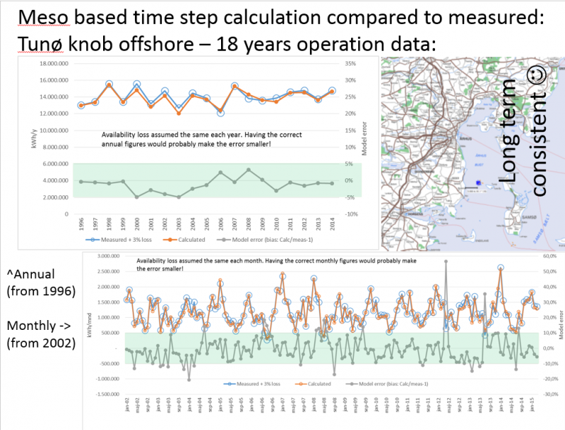
Image:Long-term consistency using Meso data

This screen shot shows how well the meso data based calculation matches measured production on a time scale of 18 years. The Tunø Knob offshore wind farm has been operating very well with few problems and a high availability during all 18 years. Thereby, it is a good validation case. It is seen that year-by-year model errors are within +/-5% and month by month within +/- 10%, apart from few months where the problems probably were related to availability issues.

Deep array wake loss model

Horns rev 1, Danish Offshore project

A more comprehensive test of the wake models, especially with deep array settings, has been performed on the Horns Rev 1 wind farm, where EMD has access to wind measurements as well as production data at a 10-minute level for one year. A calculation was set up and data loaded in the Performance Check module for detailed filtering and evaluations of the measurements against calculations on different aggregation levels. Note the deep array settings are only available for the time-step based PARK calculation, for which only the NO2005 model is available.

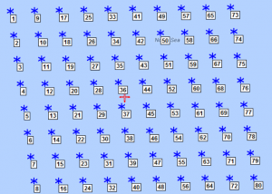
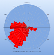
Image: Wind farm layout and the direction distribution of energy

Note the turbine orientations give the densest spacing in north, east, south and west sectors. The results are evaluated in 30-degree sectors, but calculated in 1-degree steps. The first is shown for the 360 degree calculation, meaning a full year with all data.

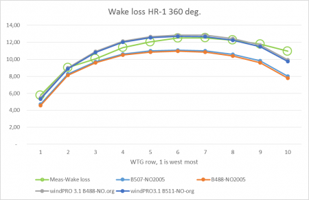
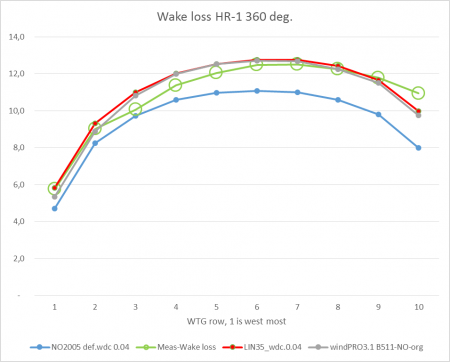
For the total wind farm, with 360 degrees and all wind speeds, the wake loss is calculated as 10.8% with the original N.O.Jensen model, exactly as measured, but with smaller deviations by turbine row. The "measured" wake losses are found by calculating with 1 year of 10-minute data and finding the ratios of measured/calculated as averages for all non-error time stamps by use of the windPRO Performance Check module. Based on the prediction error and the calculated wake loss, the measured wake loss can then be established for the sample.

Image:NO2005 variant and original N.O. Jensen model

Inclusion of mirror turbine wake (light blue line), which is new in 3.1 for NO2005 model, has almost no impact for this wind farm size. Orange line is without mirror wake.

The NO2005 variant is seen to calculate less wake loss than the original N.O.Jensen model, and too low compared to measurements.

There is a possibility to improve the NO2005 variant by using the deep array settings when calculating by time step:

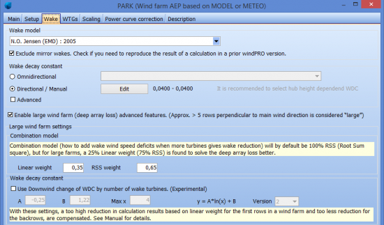
Image:The deep array loss settings for time step calculations

The linear weight of 35% is recommended. The additional option “Use downwind change of WDC by number of wake turbines are only for going down at a very detailed level. This is now in a version 2, that work somewhat differently and require new parameters. This can be used for “ultimate tuning” when very good data are available to calibrate against. See later validation tests.

Image:Using 35% linear weight in deep array model setting solve

Looking at a more detailed analysis by wind direction sector, two deep array settings are tested and compared to a baseline:

0. NO2005 standard, WDC 0.04 - the baseline.

1. Linear weight 35%, WDC 0.04.

2. Linear weight 100%, but with increased WDC from 0.04 to 0.07.

Setting 2 matches measurements almost perfect at 360 degrees, but looking at individual directions (see below), it is seen that this might not be a robust solution for all projects. For the directions where turbines are most densely spaced (north, east, south and west), an under-prediction is observed for the most wake-affected turbines. Moreover, it can be tricky to “guess” which WDC shall be used. Setting number 1 handles all directions somewhat better (i.e. there is no systematic bias), and the default WDC is used. This is likely to be a better solution when the wind farm performance is not already known.

The graphs below shows direction by direction in 30 degree sectors and illustrates how the measured/calculated ratio comes out across the average row by row, where all rows are arranged so the upwind row is row 1. The goal for a good wake model is horizontal lines in such graphs – the absolute values are less important, as they can reflect a wind speed bias.

Image: Setting 0: Calculation with default NO2005 model, WDC 0.04

Row 1, leftmost, is upwind row. Wake losses are under estimated the more downwind in the row.

Image: Setting 1: Calculation with 35% linear weight

Reasonably straight lines for all direction sectors, meaning the wake model settings work well. (almost no data from NNE and ENE may explain poor behaviour here).

Image: Setting 2: Calculation with 100% Linear weight and WDC 0.07

Wake losses are over-predicted in back rows for the direction sectors where turbines are oriented along the sector.

As observed, the more upwind the turbines (higher row numbers), the more energy under-prediction (wake loss over prediction) is seen for the east, south and west directions with 100% linear weight – this is somewhat critical. There are, due to the nature of the data, no perfect matches for any row. The north sector is not included due to very few data points in this sector. The presented case study can be concluded with no doubt that setting 1; the NO2005 with 35% linear weight is the best alternative.

The original N.O. Jensen model is not tested by direction, as the time-step based calculation concept cannot use this model and the very detailed analyses are more difficult to perform.

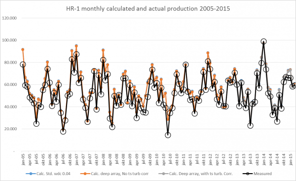
In addition, and partly for evaluation of the mesoscale time consistence, a longer period is calculated, WITHOUT filtering poor performance problems out. The results can be seen in the figure below:

Image:Monthly measured and calculated

The graph above shows partly the measured results (including availability loss and internal cabling grid loss) and partly the calculated results based on the standard WDC of 0.04. The deep array loss model alone and the deep array loss model combined with time step turbulence from mesoscale data (the last one is only from 2013, since meso data does not include turbulence before 2013). As can be seen, the difference in the three calculation models are hardly visible in the graph, but there are differences, which can be seen in the graph below:

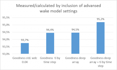
Image: Summarised result with different corrections

Summarizing the results for the different calculation setups since March 15, 2013. While the losses are assumed to be in the order of 5% (2% grid and 3% availability loss), it is assumed the most refined calculation setup provides the best result. It is noted that use of the deep array loss model calculates 0.8% higher loss and the WDC changed by time step adds a further 0.7% loss. In combination, that is an addition of 1.5% loss. This seems very little, but, with 10% wake loss with a standard calculation, it is an increase in calculated wake loss of 15%.

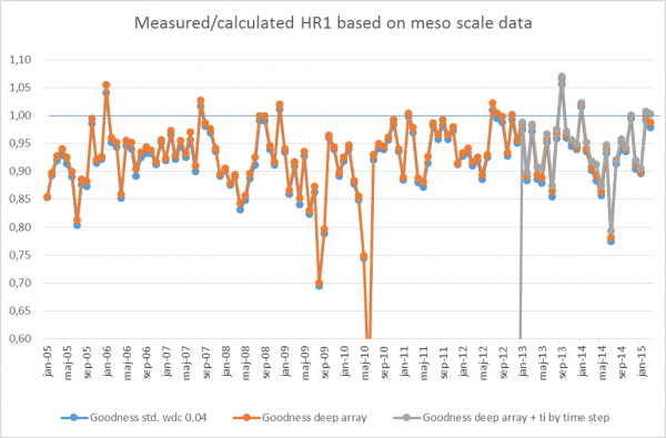
Image: Monthly ratios measured/calculated

The results shown in the above graph are shown as ratios. The reason some months have higher measured values than calculated values is because mesoscale data is not that accurate. Note that only 6 months out of 125 exhibits higher measured values than calculated. For the months with lower measured values than calculated values, it is most likely due to availability problems. Here is seen how the added wake model corrections give slightly lower calculation results (higher ratios).

The conclusion of the test with HR-1 calculations is due partly to the Mesoscale wind data performing “very precisely” (no post scaling) and partly to the deep array model modifies well. That the WDC is decided by TI adds further improvement. All in all, we recommend including all corrections. However, we must set a “warning flag” regarding the use of the meso data turbulence. Usage of the meso data in this manner has proven to provide correct results at this and a few other tested sites, but no comprehensive validation on many sites has been performed so far.

Lillgrund, Sweden offshore project

This project is special due to the dense spacing - around 3.2x the rotor diameter (RD). The main wind direction is from WSW, along the row orientation.