EMD-WRF On-Demand ICING: Difference between revisions
| Line 251: | Line 251: | ||
|colspan="4"|Data below are modelled ice model output parameters. | |colspan="4"|Data below are modelled ice model output parameters. | ||
|- | |- | ||
| | |iceInten.x | ||
| | |g/h | ||
|Water | |Ice accretion rate (intensity) [8][9] | ||
|Instantaneous | |||
|- | |||
|MIce.x | |||
|kg | |||
|Ice load on a standard cylinder [14] | |||
|Instantaneous | |||
|- | |||
|MeteoSignal.x | |||
| | |||
|Meteorological icing, iceInten.x > 10g/h [9] | |||
|Instantaneous | |||
|- | |||
|InstruSignal.x | |||
| | |||
|Instrumental Icing, MIce.x > 10g [11] | |||
|Instantaneous | |||
|- | |||
|MVD.x | |||
|m | |||
|Median Volume Diameter [6] | |||
|Instantaneous | |||
|- | |||
|LWC.x | |||
|kg/m^3 | |||
|Liquid Water Content [10] | |||
|Instantaneous | |Instantaneous | ||
|} | |} | ||
Revision as of 15:03, 4 April 2022
NOTE:
This dataset and service is currently being integrated with windPRO 3.6 (beta).
Please contact our technical specialist Marie Cecilie Pedersen (mcp@emd.dk) for more information and schedule.
We will be attending winterwind 2022 in Skellefteå, Sweden, so you are also welcome to meet with us at that event.
Introduction
EMD-WRF OD ICING is the name of EMD’s icing model. It is available as a time-series product, similar to the well known EMD-WRF OD service. The model is fully validated: A technical note with results from from recent validation study on EMD-WRF OD ICING will be available on request - and after the WinterWind 2022 and IWAIS 2022 conferences in spring 2022.
The EMD-WRF OD ICING model is configured with the following setup:
- Driven by an icing configuration of the standard EMD WRF [1] On-Demand service [2].
- Run with a spatial resolution of 3x3 km and an hourly temporal resolution.
- Using the ERA-5 reanalysis data from ECMWF as global boundary data [3], see table 2 below.
- Microphysics from Thompson scheme is used for parameterization of the cloud physics and the MYJ scheme for the planetary boundary layer physics [4], [5].
- The median volume diameter (MVD) by [6] is used, with a constant droplet concentration (Nc) of (default) 100 cm-3 and the liquid water content (LWC) in kg/m3 [7].
- Atmospheric data feeds into the standard cylinder-based model [8], [9] including melting and shedding [10].
- The WRF grid point (latitude, longitude) closest to the at mast location or site location is used as a default.
- The grid point holds a certain elevation above sea level and icing is modelled as a default for 15 heights in the vertical direction above ground level (agl.).
- The modelled ice load (kg) is used to identify hours of instrumental icing based on the industry standard thresholds of 10 g [11]. And similar from the modelled ice accretion rate (g/h), hours of meteorological icing [12] is found using the threshold of 10 g/h [9].
The final step of EMD’s modelling chain, is an estimate of the expected production loss of a site which is found by using the IEA Ice Classification system seen in Table 1 below. A wide range of climate parameters will be availabe form a model-run; the complete list of parameters are seen in the Table 2 further below.
| IEA Ice-Class |
Meteorological Icing (% of year) |
Instrumental Icing (% of year) |
Production loss (% of AEP) |
|---|---|---|---|
| 5 | > 10.0 | > 20.0 | > 20.0 |
| 4 | 5.0 - 10.0 | 10.0 - 30.0 | 10.0 - 25.0 |
| 3 | 3.0 - 5.0 | 6.0 - 15.0 | 3.0 - 12.0 |
| 2 | 0.5 - 3.0 | 1.0 - 9.0 | 0.5 - 5.0 |
| 1 | 0.0 - 0.5 | < 1.5 | 0.0 - 0.5 |
What you get and how to order?
To get pointwise-timeseries data, you need meso-credits (one credit is worth one month of data). Credits can be ordered here: http://www.emd.dk/windpro/online-ordering/
Please note, that a time period of 10 years will include the complete icing analysis, whereas shorter time periods include only raw timeseries. Complete icing analysis includes:
- Icing reports as pdfs at three hub-heights - 100m, 150m and 200m
- Including predicted AEP loss
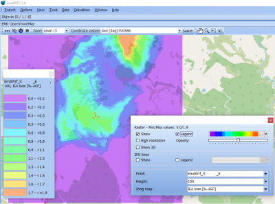
- Icing maps at three hub-heights - 100m, 150m and 200m
- IEA ice class, IEA Ice loss (% AEP) and modelled meteorological icing (icing rate > 10 g/h)
- The possibility to use your icing results and timeseries directly in your windPRO project
- Monthly, yearly and seasonal icing analysis and bin-sector analysis as csv-files
- Timeseries of raw WRF data and modelled icing
Data Availability
All EMD-WRF OD ICING is available with global spatial coverage. The temporal availability and update frequency depends on a number of factors such as availability from the boundary data providers, bandwidth and download times, as well as availability on EMD high-performance computing and storage systems. EMD-WRF OD ICING is availability with the ERA5 only, see table below.
| Dataset | First date | Most recent date |
|---|---|---|
| EMD-WRF OD (ERA5) | 1999.01.01 | 2-3 months from present day |
Set of Standard Dataset Parameters for Icing
A large quantity of useful parameters are available directly in WindPRO to aid in your analysis. The different parameters in each On-Demand ICING dataset is shown in the list below.
Unless other specification, x is the vertical heights of: 10m, 25m, 50m, 75m, 100m, 150m, 200m, 300m, 400m, 500m, 600m, 1000m.
| Parameter | Unit | Description | Type |
|---|---|---|---|
| time | UTC time stamp | ||
| psfc | Pa | Pressure at site | Instantaneous |
| msl | Pa | Pressure at mean sea level | Instantaneous |
| wSpeed.x | m/s | Wind speeds | Instantaneous |
| wDir.x | deg | Wind direction | Instantaneous |
| wSpeed.0-30mb | m/s | Wind speeds at pressure level 0-30mb. | Instantaneous |
| wDir.0-30mb | deg | Wind speeds at pressure levels 0-30mb. | Instantaneous |
| wSpeed.850hpa | m/s | Wind speeds at pressure level 850hPa. | Instantaneous |
| wDir.850hpa | deg | Wind speeds at pressure levels 850hPa. | Instantaneous |
| temperature.2 | celcius | Temperatures at height 2m | Instantaneous |
| waterTemp | celcius | Water temperature | Instantaneous |
| soilTemp.0-10cm | celcius | The temperature in the upper 10cm of the soil | Instantaneous |
| relHumidity.2 | % | Relative humidity in height 2m above ground level | Instantaneous |
| snowDepth | m | Snow depth (if present) | Instantaneous |
| vis.x | m | Visibility | Instantaneous |
| sensHeatFlux.s | w/m2 | Sensible Heat Flux at surface | Instantaneous |
| totPrecip.s | kg/m^2 | Total Precipitation at surface | 1h Accumulated |
| downShortWaveFlux.s | w/m2 | Downward shortwave irradiance at surface | 1h Average |
| totalCloudCover.a | % | Total cloud cover in atmosphere | 1h Average |
| convCloudCover.a | % | Convective cloud cover in atmosphere | 1h Average |
| 4LFTX | K | N/A | |
| rmol | 1/m | Inverse Monin-Obukhov-Length | |
| znt | m | Rougnhess length | |
| sqrtTKE.x | m/s | Wind speed given as standard deviation in m/s. Derived from the turbulent kinetic energy (TKE) | Instantaneous |
| cloudWater.x | mg/kg | Cloud water content | Instantaneous |
| cloudIce.x | mg/kg | Cloud ice content | Instantaneous |
| press.x | Pa | Pressure | Instantaneous |
| temperature.x | celcius | Temperatures | Instantaneous |
| rh.x | % | Relative humidity | Instantaneous |
| cloudBottom | m | Distance from ground level to the bottom of cloud | Instantaneous |
| cloudTop | m | Distance from ground level to the top of cloud | Instantaneous |
| waterTemp | celcius | Water temperature | Instantaneous |
| Data below are modelled ice model output parameters. | |||
| iceInten.x | g/h | Ice accretion rate (intensity) [8][9] | Instantaneous |
| MIce.x | kg | Ice load on a standard cylinder [14] | Instantaneous |
| MeteoSignal.x | Meteorological icing, iceInten.x > 10g/h [9] | Instantaneous | |
| InstruSignal.x | Instrumental Icing, MIce.x > 10g [11] | Instantaneous | |
| MVD.x | m | Median Volume Diameter [6] | Instantaneous |
| LWC.x | kg/m^3 | Liquid Water Content [10] | Instantaneous |
References
- W. C. Skamarock, J. B. Klemp, J. G. D. O. Dudhia, D. M. Barker, W. Wang and J. G. Powers, “A description of the advanced research WRF version 2,” NCAR Technical Note, Boulder, Colorado, USA, 20005.
- M. L. Thøgersen, “help.emd.dk,” EMD International A/S, 2019. [Online]. Available: https://help.emd.dk/mediawiki/index.php?title=EMD-WRF_On-Demand_and_Custom-Area. [Accessed 30 November 2021].
- ECMWF, “Advancing global NWP through international collaboration,” ECMWF, [Online]. Available: https://www.ecmwf.int/. [Accessed 23 March 2022].
- G. Thompson, P. R. Field, R. M. Rasmussen and W. D. Hall, “Explicit Forecasts of Winter Precipitation Using an Improved Bulk Microphysics Scheme. Part II: Implementation of a New Snow Parameterization,” American Meteorological Society, vol. 136, no. Monthly Weather review, pp. 5095-5115, 2008.
- Z. I. Janjic, “Nonsingular Implementation of the Mellor-Yamada Level 2.5 Scheme in the NCEP Meso model,” National Centers for Environmental Prediction, Washington, 2001.
- K. FINSTAD, E. LOZOWSKI and L. MAKKONEN, “On the median volume diameter approximation for droplet collision efficiency,” Journal of Atmospheric Sciences, vol. 45, pp. 4008-4012, 1988.
- G. Thompson, B. E. Nygaard, L. Makkonen and S. Dierer, “Using the Weather Research and Forecasting (WRF) model to predict ground/structural icing,” in International Workshop on Atmospheric Icing on Structures (IWAIS), 2009.
- L. Makkonen, "Models for the Growth of Rime Glaze Icicles and Wet Snow on Structures," Royal Society, vol. 1776, no. Ice and Snow Accretion on Structures, pp. 2913 - 2939, 2000.
- ISO, "DS/ISO 12494:2017 Atmospheric icing on structures," Danish Standard Association, København, 2017.
- K. Harstveit, “Using Metar-data to Calculate In-cloud Icing on a Mountain Site Near by the airport,” in 13th International Workshop on Atmospheric Icing on Structures (IWAIS), Andermat, Switzerland, 2009.
- K. Hämäläinen and S. Niemelä, “Production of a Numerical Icing Atlas for Finland,” Wind Energy, vol. 20, pp. 171-189, 2017.
- I. Baring-Gould, R. Cattin, M. Durstewitz, M. Hulkkonen, A. Krenn, T. Laakso, A. Lacroix, E. Peltola, G. Ronsten, L. Tallhaug and T. Wallenius, "13 Wind Energy Projects in Cold Climate 1st edition," IEA Wind Task 19, 2011.
- S. Söderberg, G. Rossitto, A. Derrick, M. Zhu and L. Gilbert, “Modelled icing losses with WICE: A blind test in France,” in Winterwind 2021, online, 2021 .