Lasten - Anhang IV: Theorie der Ermüdungslasten und LOAD RESPONSE

Zur deutschen Hauptseite | Alle deutschsprachigen Seiten

Deutsche Übersetzung folgt.

This appendix describes the fatigue design load cases, which should be considered according to the wind turbine standard IEC 61400-1 ed. 3 (2010) along with the workflow for determining fatigue loads.

Design load cases

The design load cases in IEC 61400-1 ed. 3 (2010) are developed in order to represent all significant design situations during a wind turbines design lifetime in both ultimate (extreme) and fatigue loading.

1. Power production
2. Power production plus occurrence of faults
3. Start up
4. Normal shut down
5. Emergency shut down
6. Parked (standing still or idling)
7. Parked and fault conditions
8. Transport, assembly, maintenance and repair

The design load cases which should be considered for fatigue loading are listed in the table below (see IEC 61400-1 ed. 3 (2010) for abbreviations). In LOAD RESPONSE, only design load case 1.2 is considered, since this normally is the most dominant design load case and highly dependent on the site specific wind climate parameters. However, the minor contributions from the other DLCs may be included via the DLC Other option from windPRO 3.4. This contribution should represent the expected combined fatigue contribution within the design lifetime of all the fatigue DLCs other than DLC 1.2. IEC61400-1 ed. 4 provides guidelines for the number of expected start-ups and shut-downs.

Aero-elastic simulations

Wind turbine loads are normally determined based on aero-elastic simulations of the wind turbine during the different design situations / load cases. The aero-elastic model needs, in general, input concerning:

• Site specific wind climate parameters
  • Mean wind speeds
  • Turbulence
  • Wind shear
  • Air density
  • Inflow angle
• Structural properties
  • Blade properties (length, aero-dynamics, weight, stiffness, etc.)
  • Nacelle properties (gearbox, generator, shaft, etc.)
  • Tower properties (height, weight, stiffness, etc.)
  • Foundation properties (size, stiffness, etc.)
• Control system
  • Power curve
  • Pitch system
  • Actuators
  • Control algorithms

In the aero-elastic model, a turbulence generator is used to generate a random turbulence box containing the 3-dimensional wind speed vector at different locations in the rotor plane at different time steps. The turbulence box is normally generated based on the Kaimal or Mann turbulence model. From the turbulence box, the aerodynamic force on the wind turbine at each time step is determined. This is used to determine time-series for the forces, moments and deflections in different parts of the structure, taking the structural dynamics and the control system into account.

Fatigue – Structural components

The fatigue loads for structural components (blades, tower, shaft, etc.) are normally determined by rainflow counting of the simulated time-series. The purpose of rainflow counting is to extract the stress ranges from the time-series, which is the cause of the damage of the structure. In rainflow counting, these stress ranges are extracted in a similar way as raindrops falling from a roof, hence the name rainflow counting. Compared to other methods, rainflow counting focuses on extracting the largest stress ranges in the time-series.

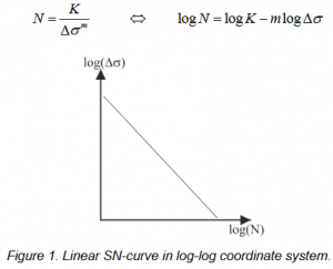
The number of cycles to failure is normally determined based on a SN-curve, which, depending on the material, can be more or less complex. However, in order to secure an easy interaction between the aeroelastic model used to determine the overall structural loading on all wind turbine components and the finiteelement models used to determine the local stresses for specific structural details, a linear SN-curve is normally used. The linear SN-curve describes the relationship between the stress range Δσ and the number of cycles to failure N, where, also, the Wöhler exponent m is introduced corresponding to the negative slope of the SN-curve. Note that the term “linear” SN-curve refers to linear in a log-log plot (see the equation and figure below).

The total damage D from the individual stress cycles extracted by rainflow-counting is normally determined by Miner’s rule for linear damage accumulation proposed by MA Miner:

where n_i is the number of cycles with stress range Δσ_i extracted by rainflow counting and N() is the number of cycles to failure for stress range Δσ_i determined from the SN-curve. If the damage is <1, the applied fatigue loading will not lead to structural failure, whereas a damage >1 will result in structural failure. In LOAD RESPONSE, the fatigue load for structural components is expressed as Damage Equivalent Load (DEL). The DEL is determined as the fatigue load which for an equivalent number of cycles n_eq will lead to the same damage as the actual load time-series for the wind turbines lifetime.

Fatigue – Mechanical components

For mechanical components, the fatigue stresses normally occur due to the interaction between different gears. This fatigue load is often characterized by the Load Duration Distribution (LDD), which describes how long time the stresses are at a given level (see, e.g.). The LDD is also dependent on the sampling frequency f and the number of time steps in the simulations with a given stress level. It is noted that the term Wöhler exponent also is used for the Load Duration Distribution, even though the same relationship to the linear SN-curve not is present.

Surrogate modelling

Fatigue loads in windPRO are approximated using surrogate models. Surrogate modelling involves creating simplified and computationally efficient models to approximate the complex relationship between input variables, such as wind conditions, and the resulting fatigue loads on the different turbine components. These models enable much quicker predictions and assessments compared to full aero-elastic simulations, facilitating a more efficient design process.

LOAD RESPONSE supports two different types of surrogate models: Central Composite Design (CCD) and Gaussian Process Regression (GPR). All generic turbine models in LOAD RESPONSE are based on the CCD, whereas for specific turbine models these can be created for either type.

Central Composite Design

The Central Composite Design, first proposed by Box & Wilson (1951). Central Composite Design was initially developed to assess second order effects in a response where interaction between different variables is present. Therefore, it constitutes a good candidate for a surrogate model, as is often the case for fatigue loads on turbines.

For each sensor in LOAD RESPONSE, a response surface is fitted at each wind speed bin in order to assess the fatigue loads accurately. In design load case 1.2, the following four wind climate parameters (variables) influence the fatigue loads:

• Effective turbulence standard deviation σ₁ (90% quantile – mean wind speed / sector dependent)
• Wind shear α (mean value – sector dependent)
• Inflow angle φ (maximum value – sector dependent)
• Air density ρ (mean value)

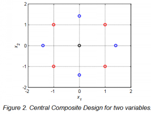
The Central Composite Design used in LOAD RESPONSE is, therefore, four dimensional. The figure below shows the principle in establishing the response surface for a two dimensional case using central composite design. The black point refers to the reference point (normally, the wind conditions for the IEC class), the blue points refer to variations of single wind climate parameters (variables) in order to estimate second order effects, and the red points refer to variations of several wind climate parameters, simultaneously, in order to estimate their interaction.

In order to setup the four dimensional response surface in LOAD RESPONSE, aero-elastic simulations for 25 combinations of the four wind climate parameters are needed at each wind speed bin. The response surface central composite design has been selected for LOAD RESPONSE, because it provides a reasonable balance between accuracy and the required number of simulations. The regression model f(x) is fitted to the response at the individual wind speed bins using linear least squares regression, where x denotes the wind climate parameters and β₀, β_i and β_ij are regression parameters.

Gaussian Process Regression

From windPRO 4.1 a more advanced surrogate model using Gaussian Process Regression (GPR) is available for specific turbine models.

Gaussian process regression is a probabilistic surrogate model which assumes the model output y(x) to be a realization of a deterministic mean defined by a regression model f(x) and a correlated stochastic process Z(x).

  y(x) ≈ f(x) + Z(x)  

The first terms f(x) to is similar to the Central Composite Design a second order regression model fitted using linear least squares. The second term Z(x) is interpolating the known residuals at the experimental design by a stationary zero mean Gaussian process fully described by its covariance.

  cov(x, x') = σ2Κ(x, x';θ)

The overall process variance σ² is assumed constant and Κ models the correlation between Z(x) and Z(x') by their inter-distance and the hyperparameters θ ∈ II₹^M. Regression coefficients β, process variance σ and hyperparameters θ is estimated by optimization, maximizing the likelihood of observing the response at the experimental design.

The GPR model in windPRO includes mean wind speed at hub height as an additional input variable compared to the Central Composite Design. Furthermore, the model can utilize random sampling of design points. This enables much greater flexibility in terms of model accuracy, as a one can increase the sampling rate at different wind conditions to increase accuracy.

For more information on GPR as a surrogate model for wind turbine fatigue assessment, see . Additionally, for a more fundamental introduction to the topic of Gaussian Process Regression, see .

Results

The damage equivalent load (DEL₀) or load duration distribution (LDD₀) is determined at each mean wind speed bin using the given surrogate model. The damage equivalent loads or load duration distribution for the full wind speed distribution (DEL / LDD) can then be determined by weighting the fatigue loads from the individual wind speed bins with the wind speed distribution:

where w(V_hub) is the weight factor determined from the wind speed distribution.

The estimated fatigue loads are presented in the following three ways in load response:

• Load (specific wind turbines)
• Load index (generic / specific wind turbines)
• Fatigue lifetime (generic / specific wind turbines)

The value of the damage equivalent load or load duration distribution is shown directly in LOAD RESPONSE for each sensor when calculations are performed for specific wind turbines implemented by manufactures. The load index is the main result, both for specific and generic wind turbines. The load index for each sensor is defined as the ratio between the fatigue load (DEL / LDD), estimated based on the site specific wind conditions, and the fatigue load (DEL_ref / LDD_ref), estimated based on the wind conditions for the considered IEC class.

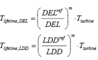
A load index <100% shows that the site specific fatigue loads are less severe than the fatigue loads for the IEC wind climate conditions. The fatigue lifetime is also determined for each wind turbine component relative to the assumed design lifetime, which, for the generic wind turbines, is assumed to T_turbine = 20 years. The fatigue lifetime will, therefore, be larger than 20 years for sensors with a load index below 100% % (below shown without DEL Other contribution).

It is noted that the fatigue lifetime does not consider other material degradation phenomena such as abrasion or corrosion.

Referenzen:

SITE COMPLIANCE & LOAD RESPONSE
SITE COMPLIANCE: Überblick ♦ Schritt-für Schritt ♦ Berechnung ♦ Ergebnisse
Hauptprüfungen: Komplexität ♦ Extremwind ♦ Turbulenz ♦ Windverteilung ♦ Windshear ♦ Neigung der Anströmung♦ Luftdichte
Andere Prüfungen: Erdbebenrisiko ♦ Temperaturbereich ♦ Blitzrate
LOAD RESPONSE: Überblick ♦ Berechnung ♦ WEA-Modelle ♦ Ergebnisse
Anhang: Gumbel Theory of Extremes ♦ Frandsen-Modell ♦ Grenzen in SITE COMPLIANCE ♦ Theorie Ermüdungslasten ♦ Sektormanagement ♦ IEC 61400-1 Ed.2 ♦ IEC 61400-1 Ed.4 ♦ Weiterbetrieb ♦ Siteres ♦ Tropical Cyclone Analysis ♦ Downscaling, Offshore-Modus & Spektralkorrektur